Introduction to R
(Part I)
Tilburg University
2024-01-11
Who am I?
- Giuseppe Arena, work as Researcher at the Department of Methodology and Statistics (TSB)
- Passionate about statistics and programming
- Background studies: statistics, biostatistics and social network analysis
- Creator and maintainer of several R packages

![]()
![]()
![]()
Goals of this workshop
![]()
![]() understanding
understanding
basic R language
![]() defining
defining
data structures
![]()
writing
functions
![]()
![]()
exploring
data
![]()
visualizing
data
![]()
running
statistical analyses

 understanding
basic R language
 defining
data structures

writing
functions


exploring
data
visualizing
data
running
statistical analyses
What is R?
Programming language, dialect of the S language, designed in the 90s by Robert Gentleman and Ross Ihaka
Framework suitable for statistical modeling , data processing, analysis, and visualization
Programming language, dialect of the S language, designed in the 90s by Robert Gentleman and Ross Ihaka
Framework suitable for statistical modeling , data processing, analysis, and visualization
Why R?
- free
- open
- simple
- interactive
- versatile
From simple to more complex analyses
Calculating the mean
mean(c(1,2.3,5,3.2,5.4,3,2.1,7,4.8,2))
Multilevel linear regression
lme4::glmer(income ~ (1|family) + condition, data = people)
mean(c(1,2.3,5,3.2,5.4,3,2.1,7,4.8,2))
lme4::glmer(income ~ (1|family) + condition, data = people)
R is widely used
![]() Academic research
Academic research
![]() Social Sciences
Social Sciences
![]() Finance and Economics
Finance and Economics
![]() Bioinformatics
Bioinformatics

 Academic research
 Social Sciences
 Finance and Economics
 Bioinformatics
Getting Started with R
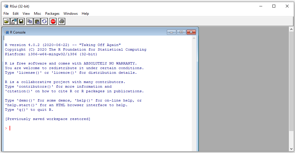
R GUI and RStudio
RStudio User Interface
Source code (syntax)
Interactive console
Environment (variables)
Graphics (plots)
R console...
... is interactive!
> "Luke"
[1] "Luke"

> 3.1416
[1] 3.1416

> 3 + 2
[1] 5

> # I am a comment (start a line with # to write any comment)

> I am not a comment
Error: unexpected symbol in "I am"
R Packages
R packages are expansions packs for R and include:
![]()
functions
adding specific functionalities
![]() documentation describing how to use the functions
documentation describing how to use the functions
![]()
data
used for the examples
R comes with base packages: base, utils, datasets, graphics, grDevices, and others
R packages are expansions packs for R and include:

functions
adding specific functionalities
 documentation describing how to use the functions
data
used for the examples
R comes with base packages: base, utils, datasets, graphics, grDevices, and others
Data Structures and Functions
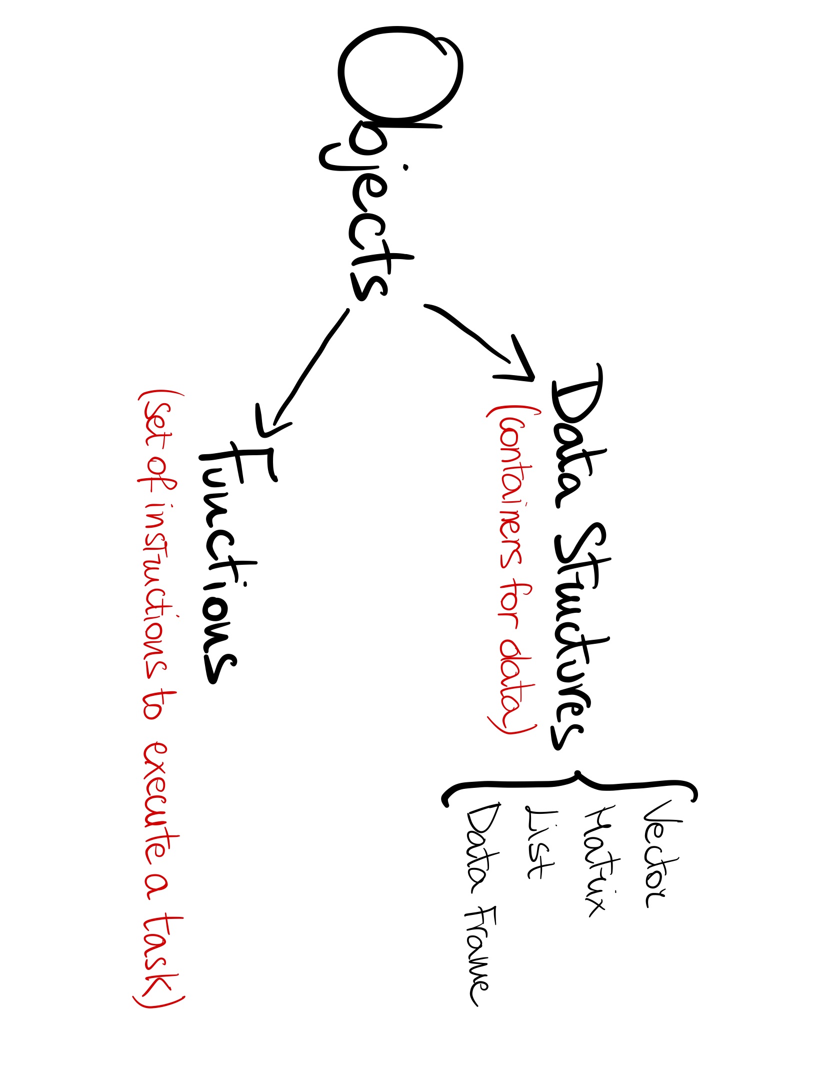
Data Structures
Data Type
Numeric
> 3.4
[1] 3.4
Character
> "workshop"
[1] "workshop"
Integer
> 15L
[1] 15
Logical
> TRUE
[1] TRUE
> FALSE
[1] FALSE
Vector
Numeric vector
> c(1.0, 2.3, 0.4, 3.1, 5.1, 4.2, 1.8)
[1] 1.0 2.3 0.4 3.1 5.1 4.2 1.8
Character vector
> c("Luke","Mark","Richard","Hannah","Paul")
[1] "Luke"  "Mark"  "Richard"  "Hannah"  "Paul"
Matrix
Numeric matrix
> matrix(data = c(1.0, 1.33, 1.66, 2.0, 2.33, 2.66,
									3.0, 3.33, 3.66), nrow = 3, ncol = 3)
     [,1] [,2] [,3]
[1,] 1.00 2.00 3.00
[2,] 1.33 2.33 3.33
[3,] 1.66 2.66 3.66
The correlation matrix is an example of numeric matrix.
List
Example of list
> list(v1 = c(1.1, 2.1, 3.1),
			 v2 = c("Luke", "Mark"),
			 m1 = matrix(c(1.1, 2.1, 3.1, 4.1), nrow = 2, ncol = 2))
$v1
[1] 1.1 2.1 3.1

$v2
[1] "Luke" "Mark"

$m1
		  [,1] [,2]
[1,]  1.1  3.1
[2,]  2.1  4.1
Data frame
Example of data frame
> data.frame(name = c("Luke", "Mark", "Hannah"),
		    		 age = c(22, 30, 29),
					   score = c(8.5, 7.5, 9.2))

				name age score
  1  		Luke  22   8.5
  2     Mark  30   7.5
  3   Hannah  29   9.2
The vectors defining the columns must have the same length.
Factor
Example of factor
> # eye color - character vector
> c("brown", "blue", "brown",
 "brown", "green", "green", "brown")
[1] "brown"  "blue"  "brown" "brown" "green" "green" "brown"

> # eye color - factor
> factor(c("brown", "blue", "brown",
 "brown", "green", "green", "brown"))
[1] brown blue  brown brown green green brown
Levels: blue brown green
Variables
Variables
Creating variables name, score and age
	> name <- c("Luke","Mark", "Hannah")
> name
[1] "Luke" "Mark" "Hannah"

> score <- c(8.5, 7.5, 9.2)
> score
[1] 8.5 7.5 9.2

> age <- c(22, 30, 29)
> age
[1] 22 30 29
Creating data frame sample_df
> sample_df <- data.frame(name = name,
														age = age,
														score = score)
> sample_df
		name age score
1   Luke  22   8.5
2   Mark  30   7.5
3 Hannah  29   9.2
You can also assign an object to a variable by using the operator '='.
name = c("Luke","Mark", "Hannah")
name = c("Luke","Mark", "Hannah")R is case sensitive
Example
> score <- c(8.5,7.5,9.2)
> score
[1] 8.5 7.5 9.2

> Score
Error: object 'Score' not found
Be careful when assigning variables' names and avoid confusion (!)
Accessing variables
Vector [ ]
> score
[1] 8.5 7.5 9.2 6.3 8.7 7.2

> # second element
> score[2]
[1] 7.5

> # 1st and 3rd element
> score[c(1,3)]
[1] 8.5 9.2
Matrix [ , ]
> example_matrix
	   [,1] [,2] [,3]
[1,] 1.00 2.00 3.00
[2,] 1.33 2.33 3.33
[3,] 1.66 2.66 3.66

> # selecting element 1st row, 3rd col
> example_matrix[1,3]
[1] 3.00

> # selecting whole 1st row
> example_matrix[1,]
[1] 1.00 2.00 3.00

> # selecting whole 3rd column
> example_matrix[,3]
[1] 3.00 3.33 3.66
Operators : and -c( )
Vector [ ]
> score
[1] 8.5 7.5 9.2 6.3 8.7 7.2

> # 1st, 2nd and 3rd element
> score[c(1:3)]
[1] 8.5 7.5 9.2

> # another way (excluding 4th,
> # 5th and 6th element)
> score[-c(4:6)]
[1] 8.5 7.5 9.2
Matrix [ , ]
> example_matrix
	   [,1] [,2] [,3]
[1,] 1.00 2.00 3.00
[2,] 1.33 2.33 3.33
[3,] 1.66 2.66 3.66

> # selecting first two rows and columns
> example_matrix[c(1,2),c(1,2)]
	   [,1] [,2]
[1,] 1.00 2.00
[2,] 1.33 2.33

> # another way
> # excluding 3rd row and 3rd column
> example_matrix[-3,-3]
     [,1] [,2]
[1,] 1.00 2.00
[2,] 1.33 2.33
Accessing List and Data frame
[[ ]] or $
List
> sample_list <- list(name = name,
	age = age,
	score = score)

> sample_list
$name
[1] "Luke"   "Mark"   "Hannah"
$age
[1] 22 30 29
$score
[1] 8.5 7.5 9.2

# accessing with $ and object name
> sample_list$name
[1] "Luke"   "Mark"   "Hannah"

# accessing with [[ ]] and object name
> sample_list[["name"]]
[1] "Luke"   "Mark"   "Hannah"

# accessing with [[ ]] and index
> sample_list[[1]]
[1] "Luke"   "Mark"   "Hannah"
Data frame
> sample_df <- data.frame(name = name,
													age = age,
													score = score)

> sample_df
   	name age score
1   Luke  22   8.5
2   Mark  30   7.5
3 Hannah  29   9.2

# accessing with $ and column name
> sample_df$name
[1] "Luke"   "Mark"   "Hannah"

# accessing with [[ ]] and column name
> sample_df[["name"]]
[1] "Luke"   "Mark"   "Hannah"

# accessing with [[ ]] and index
> sample_df[[1]]
[1] "Luke"   "Mark"   "Hannah"
Calculating with variables
Variables can be used for performing any calculation that is possible given the data structure and the data type they are assigned to.
score
[1] 8.5 7.5 9.2
addition
> score + 1
[1]  9.5  8.5 10.2
subtraction
> score - 1
[1] 7.5 6.5 8.2
multiplication
> score * 2
[1] 17.0 15.0 18.4
division
> score / 10
[1] 0.85 0.75 0.92
sum( )
> sum(score)
[1] 25.2
mean( )
> mean(score)
[1] 8.4
max( )
> max(score)
[1] 9.2
min( )
> min(score)
[1] 7.5
score
[1] 8.5 7.5 9.2
addition
> score + 1
[1] 9.5 8.5 10.2
subtraction
> score - 1
[1] 7.5 6.5 8.2
multiplication
> score * 2
[1] 17.0 15.0 18.4
division
> score / 10
[1] 0.85 0.75 0.92
sum( )
> sum(score)
[1] 25.2
mean( )
> mean(score)
[1] 8.4
max( )
> max(score)
[1] 9.2
min( )
> min(score)
[1] 7.5
Function
Defining a function
		> my_function_name <- function(arg1, arg2,
			 arg3, ...) {

	# Body of the function with
	# code to be exectuted
	# ...

	return(output) # return output object
}
- '
my_function_name' is the name of the function
- '
arg1', 'arg2' and 'arg3' are the function's arguments
- the body of the function contains the code that is executed
- '
return( )' is the statement used to specify the objects to be returned by the function
my_function_name' is the name of the functionarg1', 'arg2' and 'arg3' are the function's argumentsreturn( )' is the statement used to specify the objects to be returned by the functionExample with mean( )
The function 'mean( )' in R calculates the arithmetic mean (average) of a numeric vector
> # Define a numeric vector named 'numbers'
> numbers <- c(1,2,3,4,5,6,7,8,9,10)

> # calculate mean using 'mean( )' and assign it to 'average'
> average <- mean(x = numbers)

> # Print out 'average' variable
> average
[1] 5.5
Custom mean function
We can write our own function to compute the average of a numeric vector.
my_mean( )
> # Define custom function 'my_mean'
> my_mean <- function(x) {
		total <- sum(x) # sum of elements of x
		n <- length(x) # number of elements inside vector x
		output <- total / n # mean stored in (local) object called 'output'
		return(output) # return output object
}

# Using the custom function on the numeric vector 'numbers'
my_average <- my_mean(numbers)
> my_average
[1] 5.5
Sharing and reusing functions:
R packages
Installing and loading R packages
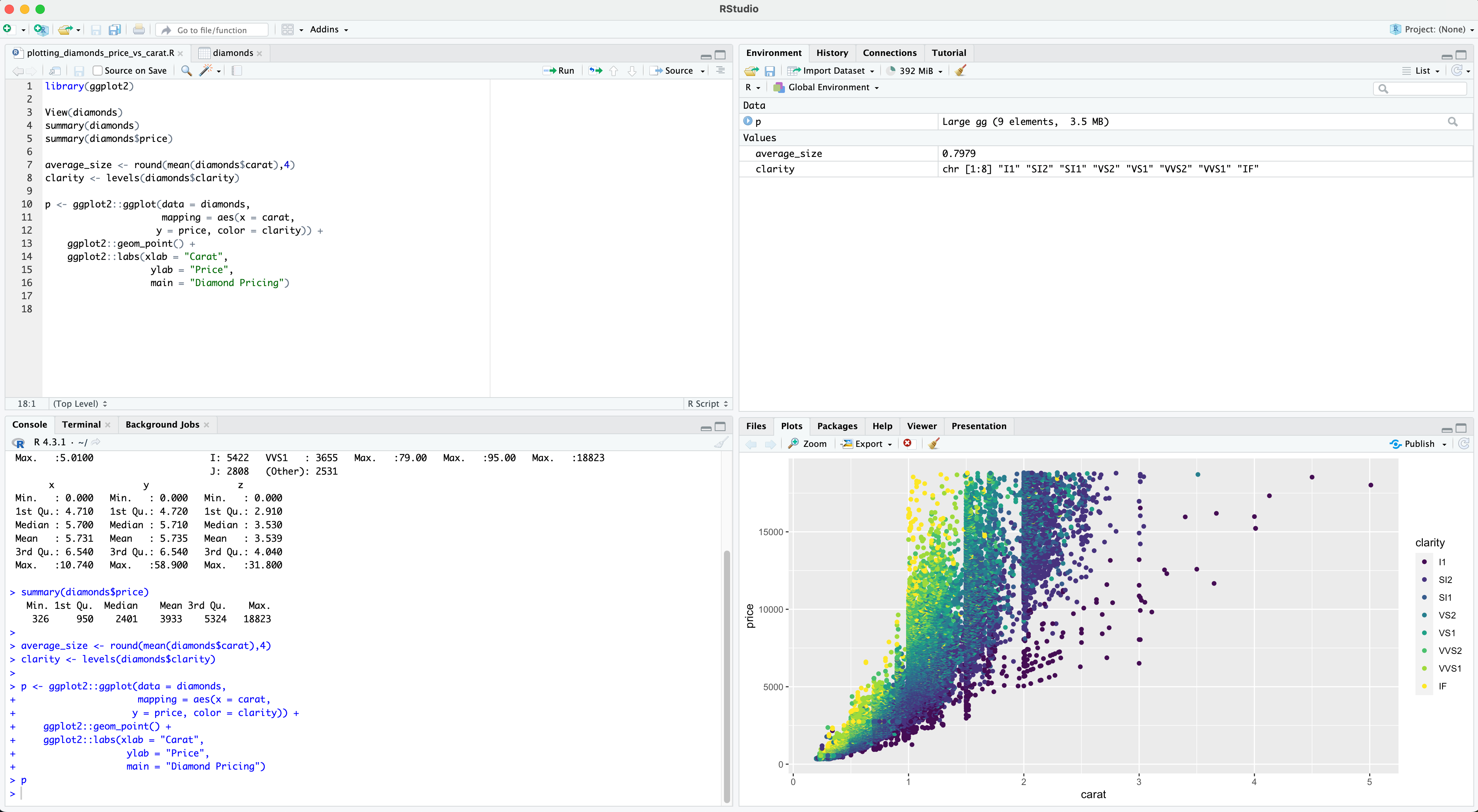
Example with 'ggplot2' package
						> # install package 'ggplot2' used for data visualization
> # (we will need it in the second part of the workshop!)
> install.packages("ggplot2")

> # NOTE:
> # at the beginning of the installation you may be asked to select
> # a mirror from which to download the package (56 is Netherlands)
> # you can choose whatever number

> # load library 'ggplot2' with library() function
> library(ggplot2)
Using functions from R packages
						> # loading library 'ggplot2'
> library(ggplot2)

> # (1) calling function 'ggplot( )' from 'ggplot2' package
> plot1 <- ggplot(data = data)

> # (2) calling function 'ggplot( )' using the syntax
> # name_package::name_function( )
> plot1 <- ggplot2::ggplot(data = data)
The syntax with : : is usually convenient when two or more loaded packages have functions with the same name
Help documentation
help( ) and ?
							> # help documentation of package "base"
> help(package = "ggplot2")

> # help documentation of function "ggplot( )" inside package "ggplot2"
> help(topic = "ggplot", package = "gglpot2")
> # or
> ?ggplot2::ggplot

> # when the library "ggplot2" is already loaded on the workspace
> ?ggplot
Warnings and Errors
A warning message refer to potential problems with the execution of a command but the execution can still proceed without being interrupted.
						> # Warning about squared root of a negative number
> sqrt(-5)
[1] NaN
Warning message:
In sqrt(-5) : NaNs produced
An error message refers to a critical issue that prevent the command from being executed. Something went wrong and the operation cannot be successfully completed.
						> # Error about a variable that has not been defined
> result <- x - 5
Error: object 'x' not found
R Workspace Management
Workspace
> ls()
[1] "age"            "data_sample"    "example_matrix" "name"
[5] "sample_df"      "sample_list"    "score"
Working directory
getwd( )
> getwd()
[1] "/Users/giuseppe"
setwd( )
> setwd("/Users/giuseppe/Desktop/")
> getwd()
[1] "/Users/giuseppe/Desktop"
Importing and exporting tabular data
Importing tabular data
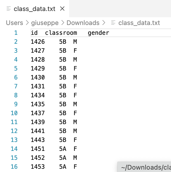
.txt file
> class_df <- read.table(
file = "/Users/giuseppe/Downloads/class_data.txt",
header = TRUE,
sep = "",
dec = "."
)
# head( ) prints out the first 6 elements of
# any data structure
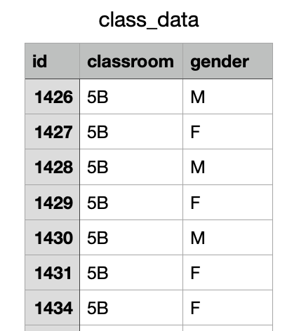
head(class_df)
id classroom gender
1 1426 5B M
2 1427 5B F
3 1428 5B M
4 1429 5B F
5 1430 5B M
6 1431 5B F
.csv file
> class_df <- read.csv(
	file = "/Users/giuseppe/Downloads/class_data.csv",
	header = TRUE,
	sep = ",",
	dec = "."
	)

head(class_df)
id classroom gender
1 1426        5B      M
2 1427        5B      F
3 1428        5B      M
4 1429        5B      F
5 1430        5B      M
6 1431        5B      F
Other useful functions for importing tabular data in R:
| Data to import | R function | package |
|---|---|---|
| .csv files that use a comma as decimal point (dec = ' , ') and a semicolon as field separator (sep = ' ; ') | read.csv2( ) | utils |
| Excel worksheets from an Excel workbook | read_excel( ) | readxl |
| read.xlsx( ) | xlsx | |
| SPSS datasets | read_sav( ) | haven |
Exporting tabular data
write.table( )
	> head(class_df)
		id classroom gender
	1 1426        5B      M
	2 1427        5B      F
	3 1428        5B      M
	4 1429        5B      F
	5 1430        5B      M
	6 1431        5B      F

	> write.table(x = class_df,
								file = "class_df.txt",
								dec = ".",
								sep = "")
Other functions for exporting tabular data:
| Type of data | R function | package |
|---|---|---|
| .csv files with comma as decimal points semicolon as field separator | write.csv2( ) | utils |
| Excel worksheet | write.xlsx( ) | xlsx |
| SPSS datasets | write_sav( ) | haven |
Summary of
Part I
Intro to R language and console (RStudio panels)
Objects: data structures and functions
Creating and accessing variables
R packages, help documentation, and workspace
Importing and exporting tabular data
Intro to R language and console (RStudio panels)
Objects: data structures and functions
Creating and accessing variables
R packages, help documentation, and workspace
Importing and exporting tabular data