Introduction to R
(Part II)
Tilburg University
2024-01-18
Welcome back!
Goals of part II
![]()
![]()
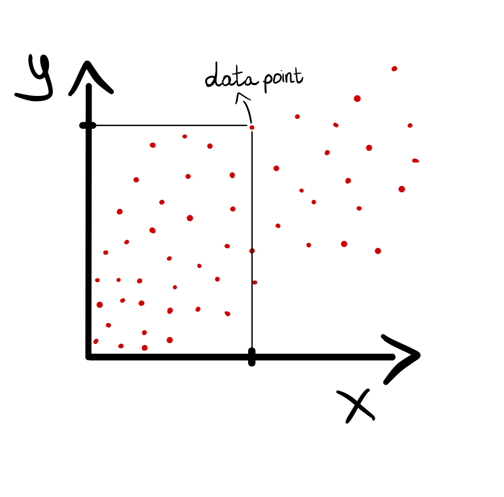
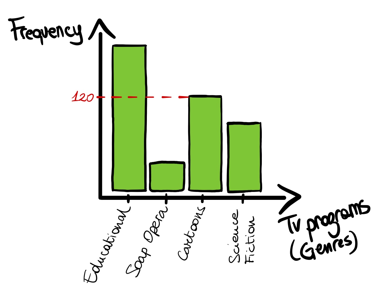
exploring
data
![]()
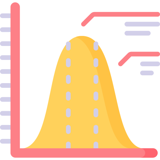
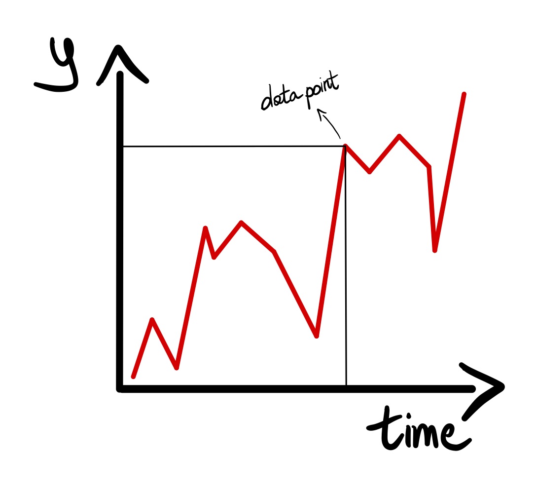
visualizing
data
![]()
running
statistical analyses


exploring
data

visualizing
data
running
statistical analyses
Data exploration
Loading data from R package into workspace
We use the dataset HolzingerSwineford1939 available inside the package lavaan.
> # install 'lavaan' package
> install.packages("lavaan", dependencies = TRUE)
>
> # loading 'lavaan' package
> library(lavaan)
This is lavaan 0.6-17
lavaan is FREE software! Please report any bugs.
>
> # load dataset in the workspace, you can check this with the function 'ls()'
> data("HolzingerSwineford1939")
>
> # use a shorter symbolic name for the dataset
> dataset1 <- HolzingerSwineford1939
>
> # re-assign the column 'sex' as a factor
> dataset1$sex <- factor(dataset1$sex)
Description of the dataset
| Variable name | Description |
|---|---|
| id | Identifier |
| sex | Gender |
| ageyr | Age, year part |
| agemo | Age, month part |
| school | School (Pasteur or Grant-White) |
| grade | Grade |
| Variable name | Description | Factor |
|---|---|---|
| x1 | Visual perception | |
| x2 | Cubes | visual |
| x3 | Lozenges | |
| x4 | Paragraph comprehension | |
| x5 | Sentence completion | textual |
| x6 | Word meaning | |
| x7 | Speeded addition | |
| x8 | Sepeeded counting of dots | speed |
| x9 | Speeded discrimination straight and curved capitals | |
Basic functions for a data.frame object
Basic functions for a data.frame object
dim( ), colnames( ), rownames( )
> # dimensions of the dataset
> dim(dataset1) # 301 rows (observations) and 15 columns (variables)
[1] 301  15
>
> # column names of 'dataset1'
> colnames(dataset1) # 'names(dataset1)' returns the same information
	[1] "id"     "sex"    "ageyr"  "agemo"  "school" "grade"  "x1"     "x2"    [...]
>
> # row names of 'dataset1'
> rownames(dataset1)
	[1] "1"   "2"   "3"   "4"   "5"   "6"   "7"   "8"   "9"   "10"  [...]
head( )
> # first six rows of a data.frame
> head(dataset1[,c(1:6)])
	id sex ageyr agemo  school grade
1  1   1    13     1 Pasteur     7
2  2   2    13     7 Pasteur     7
3  3   2    13     1 Pasteur     7
4  4   1    13     2 Pasteur     7
5  5   2    12     2 Pasteur     7
6  6   2    14     1 Pasteur     7
tail( )
> # last six rows of a data.frame
> tail(dataset1[,c(1:6)])
		id sex ageyr agemo      school grade
296 345   1    13     3 Grant-White     8
297 346   1    13     5 Grant-White     8
298 347   2    14    10 Grant-White     8
299 348   2    14     3 Grant-White     8
300 349   1    14     2 Grant-White     8
301 351   1    13     5 Grant-White    NA
Structure and summary of a data.frame
str( ) and summary( )
> # structure of the data.frame: dimensions, name and data type of each column in the data.frame
> str(dataset1[,c(1:6)])
'data.frame':	301 obs. of  6 variables:
$ id    : int  1 2 3 4 5 6 7 8 9 11 ...
$ sex   : Factor w/ 2 levels "1","2": 1 2 2 1 2 2 1 2 2 2 ...
$ ageyr : int  13 13 13 13 12 14 12 12 13 12 ...
$ agemo : int  1 7 1 2 2 1 1 2 0 5 ...
$ school: Factor w/ 2 levels "Grant-White",..: 2 2 2 2 2 2 2 2 2 2 ...
$ grade : int  7 7 7 7 7 7 7 7 7 7 ...
>
> # summary of the data.frame object (prints out a summary per each columns of the data.frame)
> ## for quantitative variables: Min - 1st Quartile - Median - Mean - 3rd Quartile - Max - NA's
> ## for qualitative (categorical) variables: frequency values
> summary(dataset1[,c(1:6)])
       id        sex         ageyr        agemo                school        grade
 Min.   :  1.0   1:146   Min.   :11   Min.   : 0.000   Grant-White:145   Min.   :7.000
 1st Qu.: 82.0   2:155   1st Qu.:12   1st Qu.: 2.000   Pasteur    :156   1st Qu.:7.000
 Median :163.0           Median :13   Median : 5.000                     Median :7.000
 Mean   :176.6           Mean   :13   Mean   : 5.375                     Mean   :7.477
 3rd Qu.:272.0           3rd Qu.:14   3rd Qu.: 8.000                     3rd Qu.:8.000
 Max.   :351.0           Max.   :16   Max.   :11.000                     Max.   :8.000
                                                                         NA's   :1
Filtering rows of a data.frame with subset( )
Filtering rows of a data.frame with subset( )
Example: subset of students from school "Pasteur", selecting only information about age (ageyr), and visual variables (x1, x2, x3).
						> # Filtering a dataset
> subset1 <- subset(x = dataset1,
+                   subset = school == "Pasteur",
+                   select = c(ageyr, x1, x2, x3))
>
> head(subset1)
	ageyr       x1   x2    x3
1    13 3.333333 7.75 0.375
2    13 5.333333 5.25 2.125
3    13 4.500000 5.25 1.875
4    13 5.333333 7.75 3.000
5    12 4.833333 4.75 0.875
6    14 5.333333 5.00 2.250
The logical operator == (double equal sign) is used for checking equality between two objects. Instead, to check whether two objects are not equal, use the operator !=.
Filtering with more conditions:
logical operators & (AND), | (OR)
Filtering with more conditions
Example 1: subset of students of the 7th grade AND from school "Pasteur", selecting only information about sex (sex), and visual variables (x1, x2, x3).
						> subset2 <- subset(x = dataset1,
+                   subset = grade == 7 & school == "Pasteur",
+                   select = c(sex, x1, x2, x3))
> head(subset2)
	sex       x1   x2    x3
1   1 3.333333 7.75 0.375
2   2 5.333333 5.25 2.125
3   2 4.500000 5.25 1.875
4   1 5.333333 7.75 3.000
5   2 4.833333 4.75 0.875
6   2 5.333333 5.00 2.250
The logical operator & (AND) compares two logical values (the one on the left and the one on the right of the symbol) and returns a TRUE only if both logical values are TRUE.
Filtering with more conditions
Example 2: subset of students from the school Pasteur AND with age less than 13 OR greater than 14 years, selecting sex (sex), age (ageyr), and visual variables (x1, x2, x3).
						> subset3 <- subset(x = dataset1,
+                   subset = (school == "Pasteur") & (ageyr < 13 | ageyr > 14),
+                   select = c(sex,ageyr, x1, x2, x3))
> head(subset3)
   sex ageyr       x1   x2    x3
5    2    12 4.833333 4.75 0.875
7    1    12 2.833333 6.00 1.000
8    2    12 5.666667 6.25 1.875
10   2    12 3.500000 5.25 0.750
11   1    12 3.666667 5.75 2.000
12   1    12 5.833333 6.00 2.875
The logical operator | (OR) compares two logical values (the one on the left and the one on the right of the symbol) and returns a TRUE if at least one of the two logical values is TRUE.
colMeans( )
						> # Function 'colMeans( )'
>
> # subset school == "Pasteur"
> subset_pasteur <- subset(x = dataset1,
+                          subset = school == "Pasteur",
+                          select = c(ageyr, x1, x2, x3) )
> # subset school == "Grant-White"
> subset_grantwhite <- subset(x = dataset1,
+                             subset = school == "Grant-White",
+                             select = c(ageyr, x1, x2, x3) )
>
> # colMeans
> colMeans(subset_pasteur, na.rm = TRUE)
	ageyr        x1        x2        x3
13.250000  4.941239  5.983974  2.487179
> colMeans(subset_grantwhite, na.rm = TRUE)
	ageyr        x1        x2        x3
12.724138  4.929885  6.200000  1.995690
Another similar function is colSums( ), which returns the sum value per each column in the data.frame (or matrix).
apply( )
						> # Applying a function (FUN) to columns/rows (MARGIN) of a data.frame/matrix (X)
>
> # using function 'apply( )' with arguments
> # X, the data
> # MARGIN, 1 for applying FUN by row, 2 for applying FUN by columns
> # FUN, the function to apply to each row or column (e.g., sd(), function to
> #                                                   calculate standard deviation)
>
> apply(X = subset_pasteur,
+       MARGIN = 2,
+       FUN = sd,
+       na.rm = TRUE)
	ageyr       x1       x2       x3
1.063318 1.185003 1.230224 1.163818
>
> apply(X = subset_grantwhite,
+       MARGIN = 2,
+       FUN = sd,
+       na.rm = TRUE)
	ageyr        x1        x2        x3
0.9681222 1.1523039 1.1112587 1.0396244
tapply( )
						> # mean of 'ageyr' per each level of variable 'school'
> tapply(X = dataset1$ageyr, INDEX = dataset1$school, FUN = mean)
Grant-White     Pasteur
	12.72414    13.25000
>
> # standard deviation  of 'x1', 'x2', and 'x3' per each level of variable 'school'
> tapply(X = dataset1$x1, INDEX = dataset1$school, FUN = sd, na.rm = TRUE)
Grant-White     Pasteur
	1.152304    1.185003
> tapply(X = dataset1$x2, INDEX = dataset1$school, FUN = sd, na.rm = TRUE)
Grant-White     Pasteur
	1.111259    1.230224
> tapply(X = dataset1$x3, INDEX = dataset1$school, FUN = sd, na.rm = TRUE)
Grant-White     Pasteur
	1.039624    1.163818
Frequency tables
table( )
						> # Contingency tables - table( )
>
> # (1) One-way contingency table of
> #     'school'
> table(dataset1$school)
Grant-White     Pasteur
		145         156
> # 145 students from "Grant-White",
> # 156 from "Pasteur"
>
> # (2) Two-way contingency table of
> #     'school' and 'sex'
> table(dataset1$school, dataset1$sex)
                 1  2
    Grant-White 72 73
    Pasteur     74 82
prop.table( )
						> # Relative frequency table - prop.table( )
> # (1) for one-way tables
> school_tab <- table(dataset1$school)
> prop.table(x = school_tab)
Grant-White     Pasteur
	0.4817276   0.5182724
>
> # (2) for two-way tables
> school_sex_tab <- table(dataset1$school,
+                         dataset1$sex)
> prop.table(x = school_sex_tab, margin = 1)
						1         2
	Grant-White 0.4965517 0.5034483
	Pasteur     0.4743590 0.5256410
Note: for one-way tables (1), the relative frequency will be calculated using the total of the table (145/301 = 0.4817 and 156/301 = 0.5183). For two-way tables (2), the user can specify which 'margin' (= 1 by rows or, = 2 by columns) to refer for the total (e.g., (2) with margin = 1).
Variance and covariance
var( )
								> # (1) var(x) to calculate variance
> # of vector 'ageyr'
> var(x = dataset1$ageyr)
[1] 1.103322
>
> # (2) var(x,y) to calculate covariance
> # beween variables 'ageyr' and 'x1'
> var(x = dataset1$ageyr, y = dataset1$x1)
[1] -0.07354743
cov( )
								> # (1) cov(x,y) to calculate
> # covariance between 'ageyr' and 'x1'
> cov(x = dataset1$ageyr, y = dataset1$x1)
[1] -0.07354743
>
> # (2) cov(x) calculates covariance matrix
> # between 'ageyr' and 'x1'
> # (supplying a data.frame to x)
> cov(x = dataset1[,c("ageyr","x1")])
			ageyr          x1
ageyr  1.10332226 -0.07354743
x1    -0.07354743  1.36289774
The standard deviation of a variable can be calculated using the function sd( ).
Correlation
cov2cor( )
								> # calculate covariance matrix with cov(x)
> cov_matrix <- cov(x = dataset1[,c("ageyr",
+                                   "x1")])
>
> # convert to correlation matrix
> # V is the input covariance matrix
> cov2cor(V = cov_matrix)
cor( )
								> # (1) cor(x,y)  calculates the correlation
> # between 'ageyr' and 'x1'
> cor(x = dataset1$ageyr, y = dataset1$x1)
[1] -0.05997699
>
> # (2) cor(x) correlation matrix of the
> # variables in a data.frame
> cor(x = dataset1[,c("ageyr","x1","x2","x3")])
        ageyr          x1         x2        x3
ageyr  1.000000 -0.059977 -0.01526 0.03718
x1    -0.059977  1.000000  0.29735 0.44067
x2    -0.015260  0.297346  1.00000 0.33985
x3     0.037179  0.440668  0.33985 1.0000
Data visualization
R packages: 'graphics' and 'ggplot2'
R packages: 'graphics' and 'ggplot2'
'graphics'
									> # plot function
> plot(x, # data
+      y, # data
+      type, # points (p), lines (l), etc..
+      main, # plot title
+      xlab, # x-axis label
+      ylab, # y-axis label
+      pch, # point style
+      lwd, # line width
+      lty, # line style
+      cex, # point size
+      col # color,
+      ...) # etc.
Input arguments avialable also for other plotting functions,
depending on the type of plot
'ggplot2'
									> # plot function with 'ggplot2'
> # concatenation of ggplot objects by '+'
> ggplot(data,  # a data.frame
+        mapping = aes(x,y)) +
+ # mapping defines an aes() object
+ # geom_point( ) add points to
+ # the ggplot object
+ geom_point(color, size) +
+ labs(title,
+      x,
+      y) +
+  theme_bw() # theme that defines the
+             # aspect of the plot
Other functions of the type geom_xzy() allow to display different types of plots
Scatter plot
plot(x, y, type = "p")
									> # Scatter plot
> plot(x = dataset1$x1,
+      y = dataset1$x2,
+      type = "p",  # 'p' = 'points'
+      main = "Scatter plot 'x1' vs. 'x2'",
+      xlab = "x1",
+      ylab = "x2",
+      pch = 1,
+      cex = 0.5,
+      col = "gray50")

geom_point( )
									> # Scatter plot with 'ggplot2'
> ggplot(data = dataset1,
+        mapping = aes(x = x1, y = x2)) +
+ geom_point(color = "gray50", size = 0.8) +
+ labs(title = "Scatter plot 'x1' vs. 'x2'",
+      x = "x1",
+      y = "x2") +
+  theme_bw()

plot(x, y, type = "p")
> # Scatter plot
> plot(x = dataset1$x1,
+ y = dataset1$x2,
+ type = "p", # 'p' = 'points'
+ main = "Scatter plot 'x1' vs. 'x2'",
+ xlab = "x1",
+ ylab = "x2",
+ pch = 1,
+ cex = 0.5,
+ col = "gray50")
geom_point( )
> # Scatter plot with 'ggplot2'
> ggplot(data = dataset1,
+ mapping = aes(x = x1, y = x2)) +
+ geom_point(color = "gray50", size = 0.8) +
+ labs(title = "Scatter plot 'x1' vs. 'x2'",
+ x = "x1",
+ y = "x2") +
+ theme_bw()
Line plot
plot(x, y, type = "l" or "b")
									> # Line plot
> # some random data
> time <- 1:20
> y <- 3.5 + time*0.4 + rnorm(n=length(time))
> plot(x = time,
+      y = y,
+      type = "l", # 'l' = 'lines'
+      main = "Line plot of 'y'",
+      xlab = "time",
+      ylab = "y",
+      col = "gray50")

geom_line( )
									> # Line plot with 'ggplot2'
> ggplot(data = data.frame(time = time, y = y),
+        mapping = aes(x = time, y = y)) +
+ geom_line(color = "gray50") +
+ labs(title = "Line plot of 'y'",
+      x = "time",
+      y = "y") +
+ theme_bw()

plot(x, y, type = "l" or "b")
> # Line plot
> # some random data
> time <- 1:20
> y <- 3.5 + time*0.4 + rnorm(n=length(time))
> plot(x = time,
+ y = y,
+ type = "l", # 'l' = 'lines'
+ main = "Line plot of 'y'",
+ xlab = "time",
+ ylab = "y",
+ col = "gray50")
geom_line( )
> # Line plot with 'ggplot2'
> ggplot(data = data.frame(time = time, y = y),
+ mapping = aes(x = time, y = y)) +
+ geom_line(color = "gray50") +
+ labs(title = "Line plot of 'y'",
+ x = "time",
+ y = "y") +
+ theme_bw()
Bar plot
barplot( )
									> # Bar plot
> frequency_school <- table(dataset1$school)
> barplot(height = frequency_school,
+         horiz = FALSE,
+         main = "Bar plot of 'school'",
+         xlab = "school",
+         ylab = "number of students",
+         ylim = c(0,
+                  max(frequency_school+10)),
+         col = "aquamarine3")
> box() # adds a square around the plot

geom_bar( )
									> # Bar plot with 'ggplot2'
> ggplot(data = dataset1,
+        mapping = aes(x = school)) +
+ geom_bar(stat = "count",
+          fill = "aquamarine3") +
+ labs(title = "Bar plot of 'school'",
+      x = "school",
+      y = "number of students") +
+ scale_x_continuous(breaks=c(11:16)) +
+ theme_bw()

barplot( )
> # Bar plot
> frequency_school <- table(dataset1$school)
> barplot(height = frequency_school,
+ horiz = FALSE,
+ main = "Bar plot of 'school'",
+ xlab = "school",
+ ylab = "number of students",
+ ylim = c(0,
+ max(frequency_school+10)),
+ col = "aquamarine3")
> box() # adds a square around the plot
geom_bar( )
> # Bar plot with 'ggplot2'
> ggplot(data = dataset1,
+ mapping = aes(x = school)) +
+ geom_bar(stat = "count",
+ fill = "aquamarine3") +
+ labs(title = "Bar plot of 'school'",
+ x = "school",
+ y = "number of students") +
+ scale_x_continuous(breaks=c(11:16)) +
+ theme_bw()
Histogram
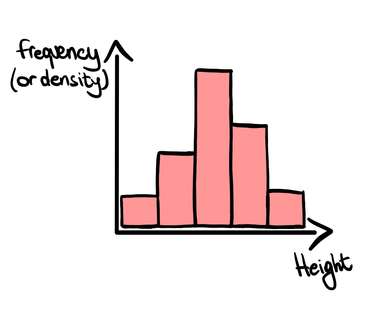
hist( )
								> # Histogram of 'x1' ('visual perception')
> hist(x = dataset1$x1,
+      freq = TRUE,
+      main = "Visual perception",
+      xlab = "value",
+      ylab = "frequency",
+      col = "lavender")
> box()

geom_histogram( )
									> # Histogram with 'ggplot2'
> ggplot(data = dataset1,
+        mapping = aes(x = x1)) +
+ geom_histogram(bins = 9,
+                fill = "lavender",
+                color = "black") +
+ labs(title = "Visual perception",
+      x = "value",
+      y = "frequency") +
+ theme_bw()

hist( )
> # Histogram of 'x1' ('visual perception')
> hist(x = dataset1$x1,
+ freq = TRUE,
+ main = "Visual perception",
+ xlab = "value",
+ ylab = "frequency",
+ col = "lavender")
> box()
geom_histogram( )
> # Histogram with 'ggplot2'
> ggplot(data = dataset1,
+ mapping = aes(x = x1)) +
+ geom_histogram(bins = 9,
+ fill = "lavender",
+ color = "black") +
+ labs(title = "Visual perception",
+ x = "value",
+ y = "frequency") +
+ theme_bw()
Density plot
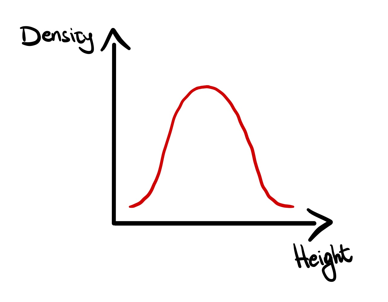
plot( x = density( ) )
								> # Density plot of 'x1'
> plot(x = density(dataset1$x1),
+      main = "Visual perception",
+      xlab = "value",
+      ylab = "density",
+      lwd = 2)

geom_density( )
									> # Density with 'ggplot2'
> ggplot(data = dataset1,
+        mapping = aes(x = x1)) +
+ geom_density(color = "black",
+              lwd = 1) +
+ labs(title = "Visual perception",
+      x = "value",
+      y = "density") +
+ theme_bw()

plot( x = density( ) )
> # Density plot of 'x1'
> plot(x = density(dataset1$x1),
+ main = "Visual perception",
+ xlab = "value",
+ ylab = "density",
+ lwd = 2)
geom_density( )
> # Density with 'ggplot2'
> ggplot(data = dataset1,
+ mapping = aes(x = x1)) +
+ geom_density(color = "black",
+ lwd = 1) +
+ labs(title = "Visual perception",
+ x = "value",
+ y = "density") +
+ theme_bw()
Box plot
boxplot('x' or 'formula' )
								> # Box plot
> # boxplot(x = , ...) # one variable only
> boxplot(
+  formula = dataset1$ageyr ~ dataset1$school,
+  main = "Age (years)",
+  xlab = "school",
+  ylab = "ageyr",
+  col = c("orange","turquoise4"),
+  horizontal = FALSE)
>
> legend("top",
+        legend = levels(dataset1$school),
+        fill = c("orange","turquoise4"))

geom_boxplot( )
									> # Box plot with 'ggplot2'
> ggplot(data = dataset1,
+        mapping = aes(x = school,
+                      y = ageyr)) +
+ geom_boxplot(mapping = aes(fill = school),
+              color = "black") +
+ labs(title = "Age (years)",
+      x = "school",
+      y = "ageyr") +
+ scale_fill_manual(values = c("orange",
+                           "turquoise4")) +
+ theme_bw()

boxplot('x' or 'formula' )
> # Box plot
> # boxplot(x = , ...) # one variable only
> boxplot(
+ formula = dataset1$ageyr ~ dataset1$school,
+ main = "Age (years)",
+ xlab = "school",
+ ylab = "ageyr",
+ col = c("orange","turquoise4"),
+ horizontal = FALSE)
>
> legend("top",
+ legend = levels(dataset1$school),
+ fill = c("orange","turquoise4"))
geom_boxplot( )
> # Box plot with 'ggplot2'
> ggplot(data = dataset1,
+ mapping = aes(x = school,
+ y = ageyr)) +
+ geom_boxplot(mapping = aes(fill = school),
+ color = "black") +
+ labs(title = "Age (years)",
+ x = "school",
+ y = "ageyr") +
+ scale_fill_manual(values = c("orange",
+ "turquoise4")) +
+ theme_bw()
geom_violin( ) with 'ggplot2'
									> # Violin plot with 'ggplot2'
> ggplot(data = dataset1,
+        mapping = aes(x = school,
+                      y = x1)) +
+ geom_violin(mapping = aes(fill = school),
+             color = "black") +
+ labs(title = "Visual perception (x1)",
+      x = "school",
+      y = "Visual perception (x1)") +
+ geom_boxplot(width=0.1) +
+ scale_fill_manual(values = c("orange",
+                              "turquoise4"))+
+ theme_bw()

> # Violin plot with 'ggplot2'
> ggplot(data = dataset1,
+ mapping = aes(x = school,
+ y = x1)) +
+ geom_violin(mapping = aes(fill = school),
+ color = "black") +
+ labs(title = "Visual perception (x1)",
+ x = "school",
+ y = "Visual perception (x1)") +
+ geom_boxplot(width=0.1) +
+ scale_fill_manual(values = c("orange",
+ "turquoise4"))+
+ theme_bw()
Correlation plot
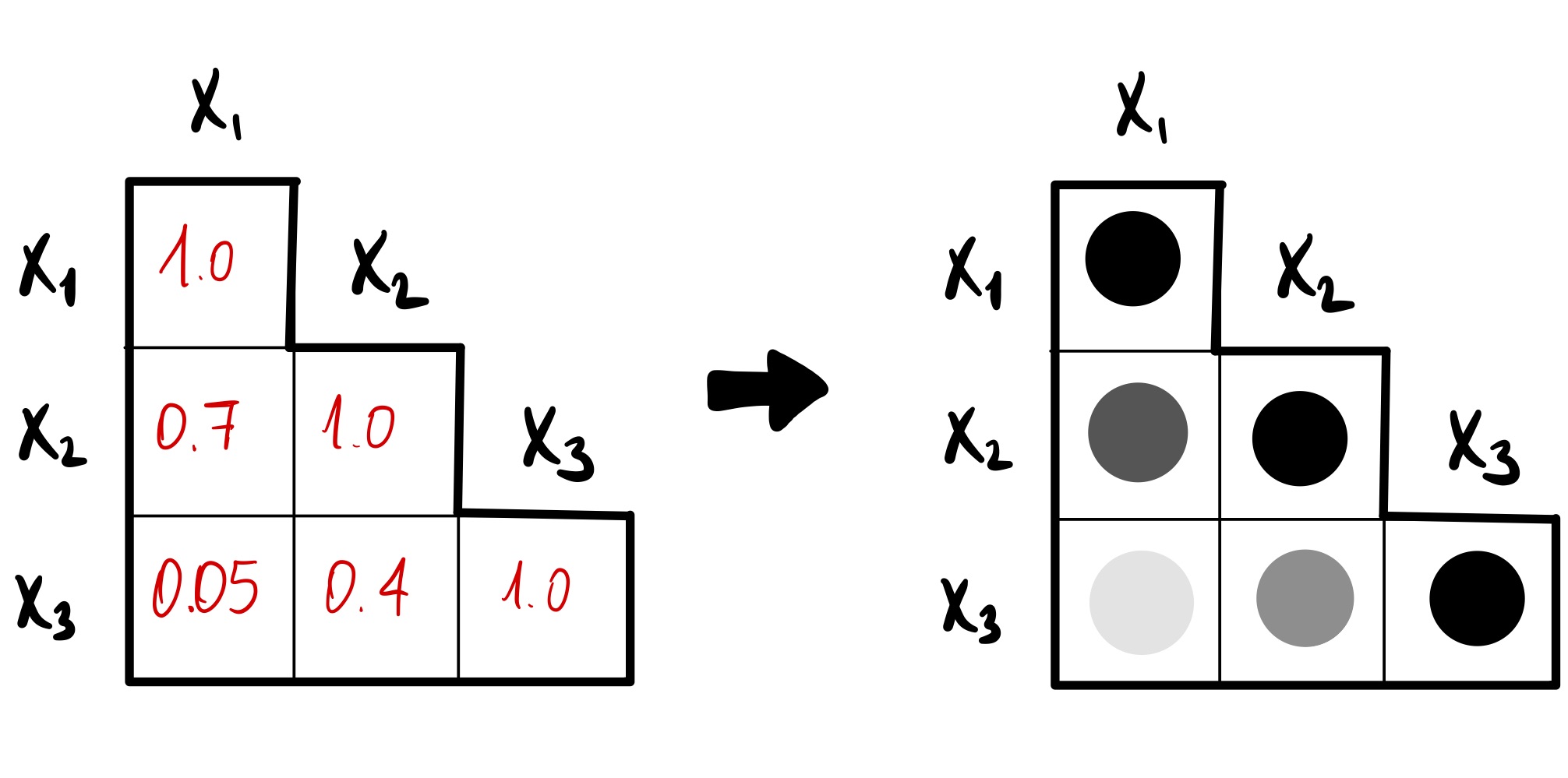
corrplot( ) with 'corrplot'
						> # Correlation plot
>
> # Install and load 'corrplot' package
> install.packages("corrplot")
> library(corrplot)
>
> # correlation matrix of x1, x2, ..., x9
> correlation_mat <- cor(dataset1[,c(7:15)])
>
> # Correlation plot with 'corrplot'
>
> # (1) method = "circle"
> corrplot(correlation_mat,
+          method = "circle",
+          type="lower")
>
> # (2) method = "number"
> corrplot(correlation_mat,
+          method = "number",
+          type="lower")


> # Correlation plot
>
> # Install and load 'corrplot' package
> install.packages("corrplot")
> library(corrplot)
>
> # correlation matrix of x1, x2, ..., x9
> correlation_mat <- cor(dataset1[,c(7:15)])
>
> # Correlation plot with 'corrplot'
>
> # (1) method = "circle"
> corrplot(correlation_mat,
+ method = "circle",
+ type="lower")
>
> # (2) method = "number"
> corrplot(correlation_mat,
+ method = "number",
+ type="lower")
Theme (ggplot2)
Applying a custom theme
					> # Theme (ggplot2)
> # (1) create ggplot object 'boxplot_x1'
> boxplot_x1 <- ggplot(data = dataset1,
+                      mapping = aes(x = school,
+                                    y = x1)) +
+ geom_boxplot(mapping = aes(fill = school),
+              color = "black") +
+ labs(title = "Visual perception",
+      x = "school",
+      y = "Visual perception") +
+ scale_fill_manual(values = c("orange",
+                              "turquoise4"))
>
> # (2) create ggplot theme 'theme_custom_1'
> theme_custom_1 <- theme_bw() +
+ theme(axis.title = element_text(size = 20,
+                                 vjust = 0.5),
+      line = element_line(linetype = "dashed"),
+      plot.title = element_text(size = 40,
+                               hjust = 0.5),
+      legend.position = "bottom",
+      legend.direction = "horizontal",
+      legend.text = element_text(size = 15),
+      legend.title = element_text(size = 15))
> # (3) add theme to the plot
> boxplot_x1 + theme_custom_1
Saving plots ...
... with RStudio
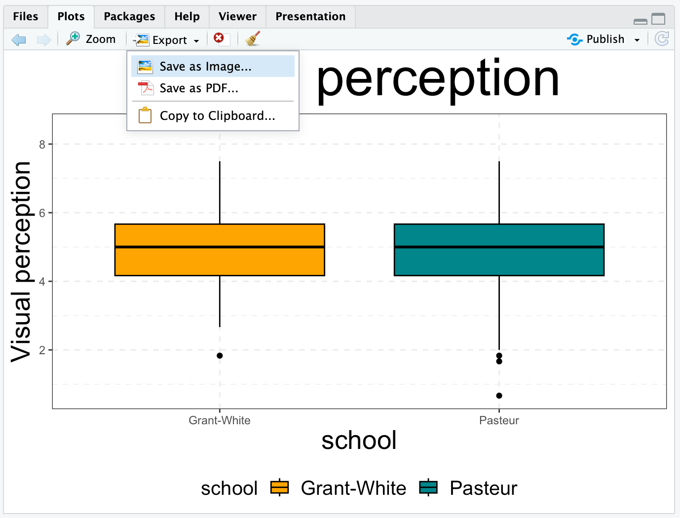
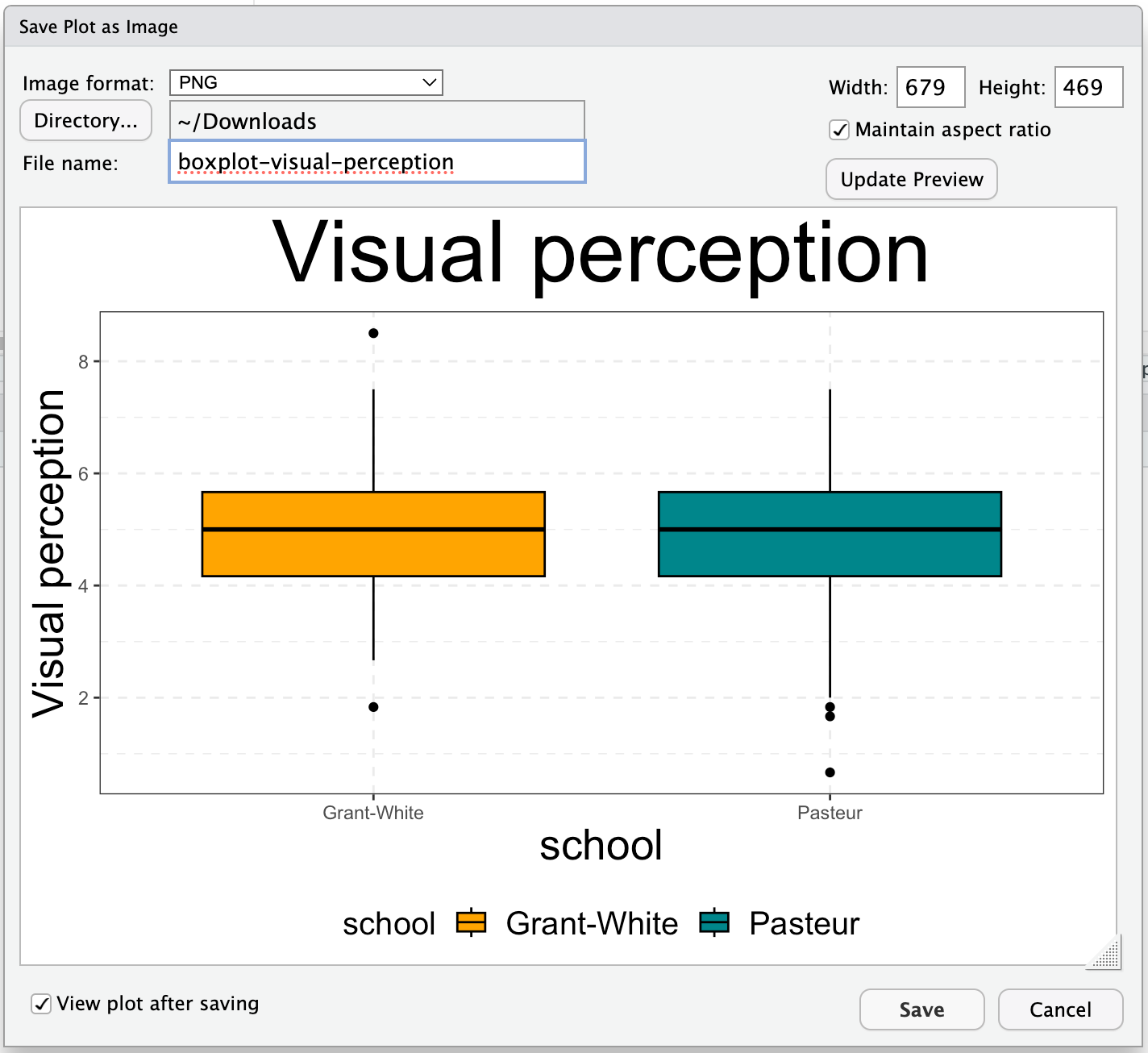
Saving plots ...
... from R console
using grDevices
								> # method (2): with 'png( )'
> # saving image into current working directory
> png(filename = "visual-perception.png",
+     width = 600,
+     height = 400,
+     units = "px")
> print(boxplot_x1 + theme_custom_1)
> dev.off() # closing R device for graphics
Other extensions are available, using the functions jpeg( ), bmp( ), tiff( ), svg( ), and pdf( )
using ggplot2
								> # method (1): with 'ggsave( )'
> ggsave(filename = "visual-perception.png",
+        width = 600,
+        height = 400,
+        units = "px")
Other extensions are available, such as .JPEG, .BMP, .TIFF, .SVG, and .PDF
Statistical Analyses in R
Linear Regression

								> # Run a simple linear regression
> lm_model <- lm(formula = x6 ~ x4,
>                data = dataset1)
> # Inspect the analysis results.
> summary(lm_model)

Call:
lm(formula = x6 ~ x4, data = dataset1)

Residuals:
     Min       1Q   Median       3Q      Max
-1.88636 -0.52249 -0.01577  0.46656  3.07582

Coefficients:
           Estimate Std. Error t value Pr(>|t|)
(Intercept)0.15613    0.12647   1.234    0.218
x4         0.66302    0.03863  17.164   <2e-16 ***
---
Signif. codes:  0 ‘***’ 0.001 ‘**’
                0.01 ‘*’ 0.05 ‘.’ 0.1 ‘ ’ 1

Residual standard error: 0.779 on 299 degrees
of freedom
Multiple R-squared:  0.4963,
Adjusted R-squared:  0.4946
F-statistic: 294.6 on 1 and 299 DF,
p-value: < 2.2e-16
Linear Regression

								> # Visualize the regression line
> ggplot(data = dataset1,
+        mapping = aes(x = x4,
+                      y = x6)) +
+ geom_point(color = "gray50") +
+ geom_smooth(method = "lm",
+             formula = y ~ x,
+             se = FALSE,
+             color = "red") +
+ theme_bw() +
+ labs(title = "Scatter plot and regression line",
+      x = "Paragraph comprehension (x4)",
+      y = "Word meaning (x6)")
Diagnostics plot
								> # Model diagnostics
> # par() to set grid 2x2 with mfrow()
> par(mfrow=c(2,2))
>
> # plot of 'lm' object
> plot(lm_model,
+      cex = 0.8, # size of the points
+      pch = 19,  # point style
+      col = rgb(red = 127,
+                green = 127,
+                blue = 127,
+                alpha = 90,
+                maxColorValue = 255), # color
+      lwd = 2) # line width

Multiple Linear Regression
						> # Run a multiple linear regression
> lm_multiple <- lm(formula = x1 ~ x2 + x3 + x4,
>                   data = dataset1)
>
> # Inspect the analysis results.
> summary(lm_multiple)

Call:
lm(formula = x1 ~ x2 + x3 + x4, data = dataset1)

Residuals:
    Min      1Q  Median      3Q     Max
-3.6957 -0.6529  0.1000  0.6616  2.3413

Coefficients:
            Estimate Std. Error t value Pr(>|t|)
(Intercept)  2.40878    0.31567   7.631 3.20e-13 ***
x2           0.13247    0.05133   2.581   0.0103 *
x3           0.35936    0.05349   6.718 9.38e-11 ***
x4           0.29789    0.04946   6.023 5.04e-09 ***
---
Signif. codes:  0 ‘***’ 0.001 ‘**’ 0.01 ‘*’ 0.05 ‘.’ 0.1 ‘ ’ 1

Residual standard error: 0.979 on 297 degrees of freedom
Multiple R-squared:  0.3039,	Adjusted R-squared:  0.2968
F-statistic: 43.21 on 3 and 297 DF,  p-value: < 2.2e-16
Structural Equation Models (SEM)
> library(lavaan)
Multiple Linear Regression in SEM framework
Model specification and estimation
									> # (1) specify model, same as with lm()
> model <- "x1 ~ 1 + x2 + x3 + x4"
> # (2) run estimation
> lm_sem_model <- sem(model = model,
+                     data = dataset1)
Summary
									> summary(lm_sem_model) # (3) inspect results
Estimator                                         ML
Optimization method                           NLMINB
Number of model parameters                         5
Number of observations                           301

Model Test User Model:
Test statistic                                 0.000
Degrees of freedom                                 0

Parameter Estimates:
Standard errors                             Standard
Information                                 Expected
Information saturated (h1) model          Structured

Regressions:
				Estimate  Std.Err  z-value  P(>|z|)
x1 ~
x2                0.132    0.051    2.598    0.009
x3                0.359    0.053    6.763    0.000
x4                0.298    0.049    6.064    0.000

Intercepts:
				Estimate  Std.Err  z-value  P(>|z|)
.x1                2.409    0.314    7.682    0.000

Variances:
				Estimate  Std.Err  z-value  P(>|z|)
.x1                0.946    0.077   12.268    0.000
SEM framework with three latent variables
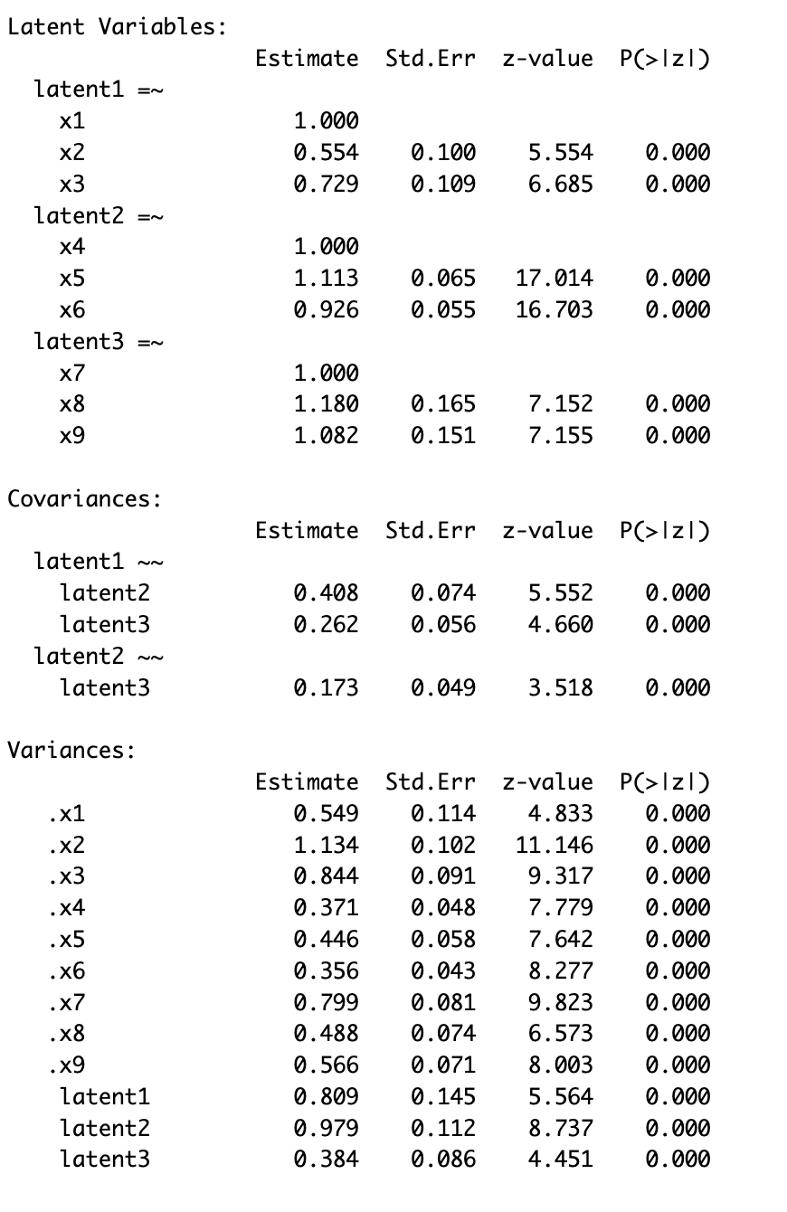
SEM framework with three latent variables
Model specification and estimation
								> # (1) Specify SEM model with three latent variables.
> model_2 <- "
+     # Latent variables
+     latent1 = ~ x1 + x2 + x3
+     latent2 = ~ x4 + x5 + x6
+     latent3 = ~ x7 + x8 + x9
+
+     # Covariance between latent variables
+     latent1 ~~ latent2
+     latent1 ~~ latent3
+     latent2 ~~ latent3
+ "
> # (2) Run the analysis
> sem_model_2 <- sem(model = model_2, data = dataset1)
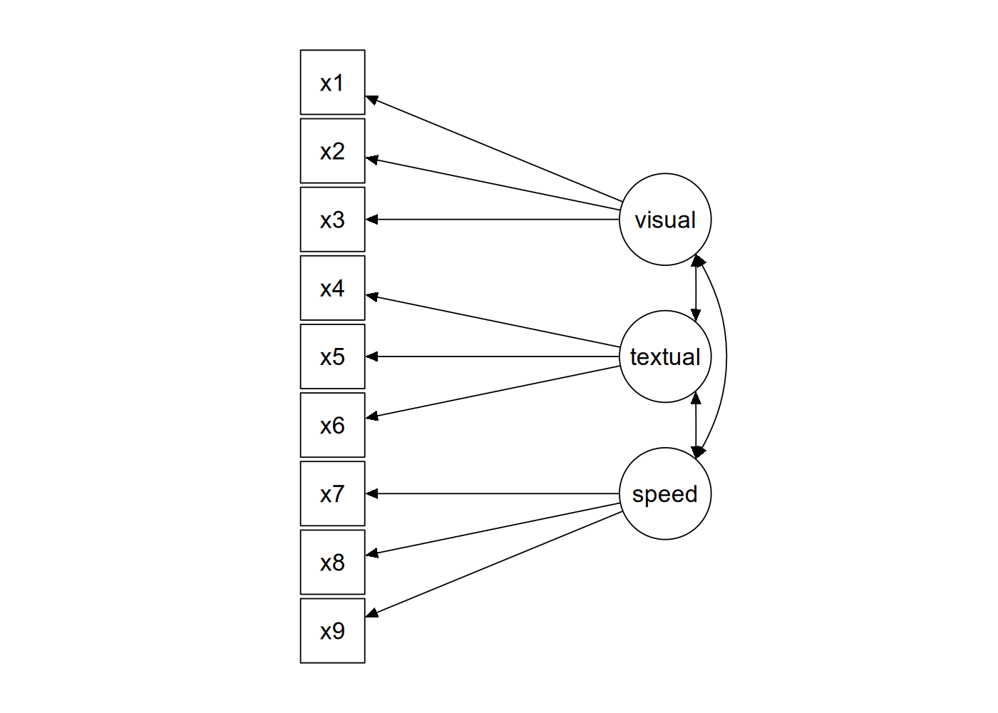
content inspired by tutorial at lavaan.ugent.be/tutorial/cfa.html
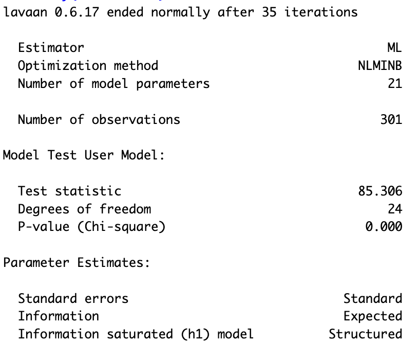
Summary SEM with latent variables
								> # summary with fit measures
> summary(sem_model_2)
> round(
+     fitMeasures(sem_model_2)[c("chisq",
+                                "df",
+                                "pvalue",
+                                "cfi",
+                                "rmsea",
+                                "srmr")], 3)
	chisq     df pvalue    cfi  rmsea   srmr
85.306 24.000  0.000  0.931  0.092  0.065
+ # print out more fit measures with
+ # summary(sem_model_2, fit.measures = TRUE)
Visualize SEM model
> library(semPlot)
Visualize SEM model
								> # Plot the SEM model with three latent variables
> semPaths(sem_model_2,
+          what = "path",
+          whatLabels = "est")

Linear Mixed-Effects Models
> library(lme4)
Random Intercept
Random intercept per school: model specification and estimation
								> # Fit a linear mixed-effects model with
> # random intercepts for school
> lme_model <- x6 ~ 1 + (1|school) + sex +
+                   ageyr + x4 + x5
> model <- lmer(formula = lme_model, data = dataset1)
> summary(model)
\[ \text{random intercept} \\ \text{per school:} \\ (1 | \text{school} )\]
Summary of the model
						Linear mixed model fit by REML ['lmerMod']
Formula: x6 ~ 1 + (1 | school) + sex + ageyr + x4 + x5
Data: dataset1
REML criterion at convergence: 661.6
Scaled residuals:
	Min      1Q  Median      3Q     Max
-2.2242 -0.6463 -0.0017  0.6048  3.4045

Random effects:
	Groups   Name        Variance Std.Dev.
	school   (Intercept) 0.001672 0.04089
	Residual             0.498582 0.70610
Number of obs: 301, groups:  school, 2

Fixed effects:
				Estimate Std. Error t value
(Intercept) -0.370401   0.582357  -0.636
sex2        -0.134552   0.083085  -1.619
ageyr       -0.006922   0.040591  -0.171
x4           0.368365   0.051866   7.102
x5           0.365919   0.047045   7.778

Correlation of Fixed Effects:
		(Intr) sex2   ageyr  x4
sex2  -0.202
ageyr -0.965  0.152
x4    -0.044 -0.107  0.035
x5    -0.260  0.058  0.112 -0.719
Note: p-value's are not reported in the summary. The 'lmerTest' package runs with the function lmerTest : : lmer( ) (same name as in 'lme4' package) returns the p-value's (this is only available for Linear Mixed-Effects Models, not for Generalized Linear Mixed-Effects Models).
Diagnostics
								> # Diagnostics of the model
>
> # Homoscedasticity of residuals
> plot(lme_model,
+      pch = 19,
+      cex = 0.8,
+      main = "Residuals",
+ )
>
> # normality - Q-Q plot
> qqnorm(residuals(lme_model))
> qqline(residuals(lme_model))


Mixed-Effects Model
Consider the variables: intercept, id (student), school, sex, x1, x2 and x3. Assume that for each student the abilities x1, x2, and x3 are measured multiple times.
| Effect | Model specification (formula) |
|---|---|
| random intercept per school | x1 ~ 1 + (1|school) |
| random intercept per school and sex | x1 ~ 1 + (1|school:sex) |
| fixed and random slope of x2 per student | x1 ~ x2 + (x2|id) |
| fixed and random slope of x2 and x3 per student | x1 ~ x2 + x3 + (x2 + x3|id) |
Summary of
Part II
Data exploration
Data visualization (with 'graphics' and 'ggplot2')
Structural Equation Models with 'lavaan' package
Linear Mixed-Effects models with 'lme4' package
Data exploration
Data visualization (with 'graphics' and 'ggplot2')
Structural Equation Models with 'lavaan' package
Linear Mixed-Effects models with 'lme4' package
Thanks for taking part in this workshop!
Happy R coding!

Resources
R coding:
Data visualization:
SEM with 'lavaan':
Linear Mixed-effects models:
R coding:
Data visualization:
SEM with 'lavaan':
Linear Mixed-effects models: